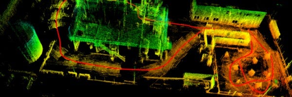
Simultaneous Localization and Mapping

You can find my final code and result here

One of the most important part of a self driving car is know where it is located at any given time. However, it is hard to get an accurate position since the sensors has inherent error usually due to the technology (such as RADAR and LiDAR). For instance, GPS is rated for +/- 1m (3 ft) but 1 m error is enough for the car to hit things accidentally. This was systemic problem when NASA was developing rocket/missile controls. The error within the sensor varied too much where the missiles could not control itself correctly as intended.

Solution

One solution to this problem is to use a Kalman filter. There are many great resources online that explain the theory and application of the Kalman filter so I will be mainly explaining my key takeaways that allowed me to understand it better. Kalman filter find it’s root from Bayesian statistic. One of the most important effect of the Bayes rule is that the more measurements you have for a given time, the lower the variance (more accurate) for your final measurement. Essentially, two (or more) noisy measurements will give you one (relatively) accurate measurement.

The Kalman filter involves two steps that runs perpetually:

1) Measurement Update 2) Motion Update

Measurement Update

Like the name implies, the measurement update is where you use the sensors to determine where you are. For instance, a self driving car can use GPS and wheel encoder to determine an approximate location. The raw measurement tends to be noisy but the variance can be greatly reduced using the Bayes rules using information that was obtained from the previous measurement (this will make more sense later).

Motion Update

After the measurement update, you move the self driving car and predict the location of the self driving car. I use the word predict because the location is usually calculated rather then measured. Therefore, in order to perform this step, the state space has to be fully defined. This is just fancy way of saying that the physics of the system must be understood and defined. For instance, the position motion update is usually predicted using the velocity of the car that can be measured using an IMU or speedometer. Since we know the velocity, we can use our high school physics knowledge to predict the position.

Source

This part is where the magic happens for the Kalman filter. By using the Bayes Rule, we can combine the measurements from the measurement step (the first posterior in the image) and the prediction from the motion step (the prior from the image) to get an accurate final result which will be the posterior used in the next motion update step. This shows you the powerful application of Bayesian statistics.

Extended Kalman Filter

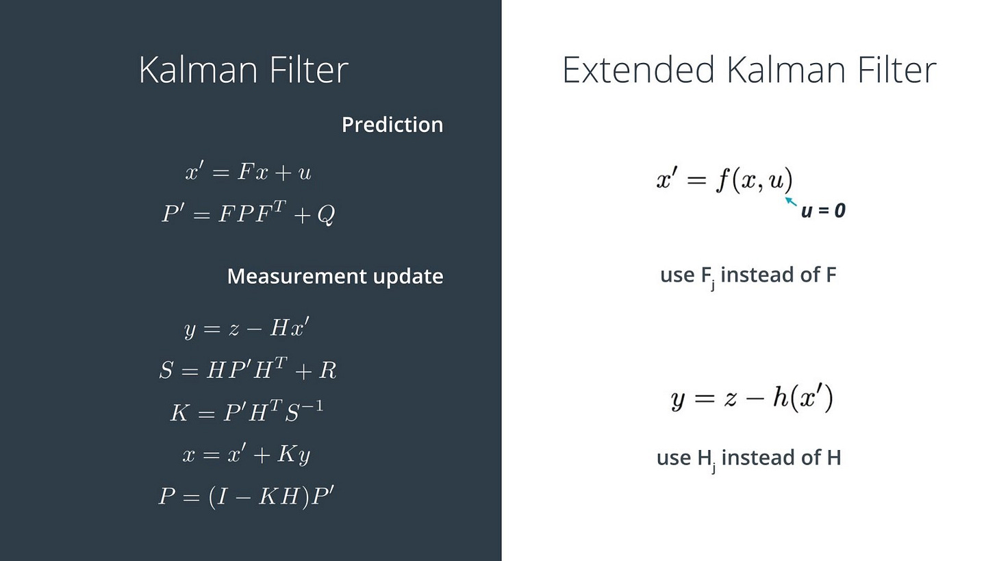
The extended Kalman filter (EKF) is the nonlinear version of a Kalman filter. I will not go into the math but the reason why EKF can accomdate for nonlinear functions is during the motion update phase, the state is linearized using an intermediate function (h(x’) shown in the image) that is usually defined using Taylor expansion. This makes the math a bit more complex but can be easily solved using the Jacobian matrix when programming it.

Unscented Kalman Filter

If you want a more thorough and good explanation, please read this medium post by Harveen Singh

I have been told that name for Unscented Kalman filter (UKF) stems from the idea that a UKF is a Kalman filter that doesn’t “stink” (or sucks and terrible for non-native English speakers). The UKF is similar to an EKF where it can account for nonlinear functions but takes it one step further which gives it better accuracy.

An EKF has induced error because when it maps it Gaussian distribution when it converts the non-linear to linear function, a lot of information can be lost. To alleviate this problem, UKF keeps track of data points in the distribution called sigma points. These points are important because you can gauge the effectiveness of the approximation. With this additional data, the final variance of the measurement is much more accurate since information from the previous step is retained better. Also, the sigma points alleviate the importance of the first measurement point which can cause an EKF to diverge.

The four additional steps for a UKF is the following:

1) Generate sigma points 2) Augment them during the nonlinear to linear process 3) Predict where the sigma points should be and compare them to how they are augmented 4) Update the measurement Gaussian distribution

Putting it all together

For a self driving car application, the UKF is usually used for the senor fusion between RADAR and LiDAR data. The main reason is because RADAR gives relative velocity data where LiDAR gives positional data. By using the UKF, the measurement of the position of your car will be much more accurate.